Gear Hashing for Content Defined Chunking

Published on 2023-03-09 to joshleeb's blog

In this post we’ll take a detailed look at Gear Hashing for Content-Defined Chunking (CDC). If you haven’t come across the term “CDC”, then take a look at the first post in this series that provides an introduction to this topic.

As a quick refresher, the core problem we need to solve for CDC is determining chunk boundaries based on a sequence of bytes. This is generally split into two stages.

Hash a window of bytes to produce a digest (fingerprint); then
Check if we have found a chunk boundary with the hash judgment function.

We’ll see how Gear Hashing defines functions for both fingerprinting and judging the hash.

Gear Hashing

Gear Hashing was first introduced in the Ddelta paper [1] as a response to the time-consuming nature of Rabin-based chunking. Here, the hashing function is defined by the following formula.

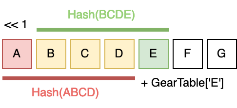
$$FP_i = (FP_{i-1} \ll 1) + GearTable[B_i]$$

$FP_i$ is the fingerprint at position $i$ in the byte sequence. To calculate the fingerprint, we take the previous fingerprint $FP_{i-1}$ and left-shift it by 1 bit. Then, we add a value from the $GearTable$ that corresponds to the byte at the current position, $B_i$.

This hashing function perfectly fits the definition of a rolling hash. The left-shift has the effect of subtracting information from the previous fingerprint while the addition adds more information based on the current byte. Together these operations form a rolling window across the byte sequence.

Note that the left-shift is only clearing one bit, specifically the most-significant bit (MSB), from the previous fingerprint and so by adding another 64 bits to form the new fingerprint it is possible to see an overflow. To avoid this we’ll use wrapping addition. Here’s what it looks like in Rust.

fn consume(fp_prev: u64, byte: u8) -> u64 {
    (fp_prev << 1).wrapping_add(GEAR_TABLE[byte as usize])
}

The last piece we need to discuss is the GearTable.

A good hash function must have a uniform distribution of hash values regardless of the hashed content [1]. And since the byte sequence is the content being hashed, the GearTable must provide that aspect of randomness we need for this to be a good hash function.

And in fact, that’s exactly how the Ddelta paper [1] defines the GearTable.

GearHash employs an array of 256 random 32-bit integers to map with the ASCII values of the data bytes in the sliding window.

The values that make up the GearTable can be anything, so long as they’re sufficiently random. The more random the GearTable, the more uniform the distribution of hash values will be produced from the Gear Hash. In our implementation we’ll go with 64 bit random values since we want a 64 bit hash.

static GEAR_TABLE: [u64; 256] = [
    0xb088d3a9e840f559, 0x5652c7f739ed20d6, 0x45b28969898972ab,
    0x6b0a89d5b68ec777, 0x368f573e8b7a31b7, 0x1dc636dce936d94b,
    0x207a4c4e5554d5b6, 0xa474b34628239acb, 0x3b06a83e1ca3b912,
    ...
];

And that’s the fingerprinting part of Gear Hashing done. It looks simple, almost too simple. Well is it?

That hashing functions you might be used to seeing, such as MD5 and the SHA family, are cryptographic hash functions. For a hash function to be considered cryptographic it needs to have specific properties that prevent attack vectors that might be present in non-cryptographic hashes. For example, given some hash value H, it should be difficult to find some message m such that H = hash(m). Gear Hashing does not meet this requirement.

But we’re not worried about security here. We care about having a fast (very fast) hash function that allows us to find patterns in the content we’re hashing. And Gear Hash is very fast. There are only three operations: 1 ADD, 1 SHIFT, and 1 ARRAY LOOKUP. For a quick comparison, Rabin fingerprinting has 1 OR, 2 XORs, 2 SHIFTs, and 2 ARRAY LOOKUPs [1].

Hash Judgment Function

Now that we know how to produce a digest, we need a way to check if the fingerprint is a chunk boundary. Turns out this is even simpler than the hashing function. From the Ddelta paper [1].

Gear-based chunking determines the chunking boundary by checking whether the value of the N MSBs of the Gear hash is equal to a predefined value.

We’ll call this predefined value the mask. The value of this mask directly influences the average size of the chunks produced following the formula N = log2(M) for the desired average chunk size M.

For example, say we want to produce chunks that are 8KiB, the size used in LBFS [2]. Using the formula log2(8192) = 13, we can use a mask with the 13 most-significant bits set to 1, and the remaining bits zeroed out.

We’ll soon see how this works in practice, but in theory this formula is derived from the probability each bit of the fingerprint will be a 1 or a 0. Assuming the Gear Hash produces random values with a uniform distribution, each bit has an even probability of being on or off. So the probability of the 13 MSBs being on is (1/2)^13 = 1/8192. That means, each bit has a 1 in 8192 chance of being a chunk boundary, or in other words, after consuming 8192 bits we should’ve produced a new chunk.

Here’s how the hash judgment function is implemented.

fn is_chunk_boundary(fp: u64, mask: u64) -> bool {
    fp & mask == 0
}

Note that by ANDing the fingerprint and the mask, we don’t care about what the lower 51 bits are in the fingerprint and so this doesn’t affect the probability of finding a chunk boundary.

Putting Gear Hashing to the Test

Let’s chunk up a fairly large bit of text, the complete works of Shakespeare (hosted here by MIT) which clocks in at 5.4MB. We’ll start by using the 13 MSB mask which should give us an average chunk size of 8KiB.

All the code used to produce these results is hosted at here on Sourcehut. If you’ve cloned the repository and would like to follow along, the chunker example can be run with cargo r --example chunker. In this post we will elide this as ./chunker. You can also run this with RUST_LOG=debug to get some extra information as the chunks are being produced.

$ ./chunker data/shakespeare.txt chunks/
ChunkStats { count: 647, total_len: 5447521 }

On this first run, the chunker produced 647 chunks with an average chunk length of 8420 bytes. That’s not far off from our desired chunk length of 8192 bytes (+2.78%)

However things aren’t all that great. If we inspect the sizes of each of the chunks we’ll see a whole assortment of values. Let’s plot them on a histogram.

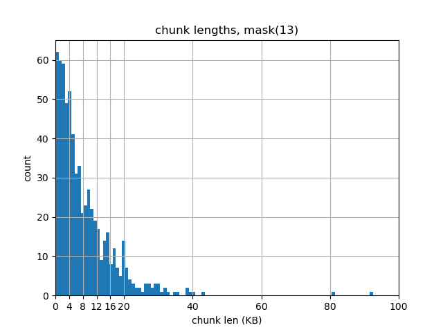
Here we see a lot of chunks that are greater than 16KiB (13.76%), and even more that are less than 4KiB (38.49%). We even have two chunks that are larger than 80KiB!

Changing the Mask

Let’s blow away the chunks/ directory and change the mask so that it has 11 MSBs set to 1 rather than 13. This should give us an average chunk length of 2KiB.

$ rm -rf chunks/
$ ./chunker data/shakespeare.txt chunks/
ChunkStats { count: 2636, total_len: 5447486 }

Again, it’s not far off. The average chunk length is 2067 bytes which is a difference of +0.98%.

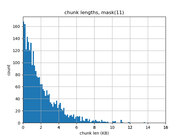
This histogram looks a little better. The largest chunk is less than 14KiB, but we still have a significant number of chunks that are less than 2KiB.

Checking Boundary Shift

So the chunk length is a bit all over the place, but how does Gear Hashing fair with the boundary shift problem?

To test this, we’ll set our mask back so we have a desired average chunk length of 8KiB (i.e: 13 MSBs set to 1) and produce some fresh chunks.

$ rm -rf chunks/
$ ./chunker data/shakespeare.txt chunks/

Then we modify shakespeare.txt by inserting “x” at the beginning of the file.

$ { echo -n 'x'; cat data/shakespeare.txt; } > data/shakespeare_x.txt

And rerun the chunker with the modified data and the chunks/ directory intact.

$ ./chunker data/shakespeare_x.txt chunks/
ChunkStats { count: 1, total_len: 850 }

Fantastic! Gear Hashing picked up that only the first chunk was modified, and so only one new chunk needed to be produced. And that the rest of the file was unchanged and so we could reuse the existing chunks.

In this test, albeit rather contrived and limited, the Gear Hash chunker deduplicated almost all the content. So it’s safe to say that Gear Hashing doesn’t suffer from the boundary shift problem. If this were FSC, then all chunks would be recreated and we would have no deduplication.

The Problem with Gear Hashing

As we saw with the histograms above, the biggest problem with Gear Hashing is the non-uniformity of chunk lengths. With CDC we don’t expect all chunks to have the exact same length, but we’d like them to all be in the same ballpark, and not have almost 40% of chunks less than half the desired average size.

It doesn’t show up in the deduplication test we just ran, but the impact of having chunk lengths all over the place is on the deduplication ratio. The FastCDC [3] paper explains that this issue stems from the hash judgment stage, where the sliding window is very small, leading to more chunking boundaries being found.

The sliding window size of the Gear-based CDC will be equal to the number of bits used by the mask value. Therefore, when using a mask value of 2^13 for the expected chunk size of 8KiB, the sliding window for the Gear-based CDC would be 13 bytes.

Note that the sliding window is 13 bytes with a mask containing the 13 MSBs set to 1. This is because when hashing each new byte, we shift the hash by 1 bit. And so, during the hash judgment phase, the mask looks at information in the fingerprint that has been gathered from the most recent 13 bytes.

The FastCDC paper [3] has an in-depth analysis of this. For some datasets, Gear-based CDC shows a deduplication ratio that is consistently less than the deduplication ratio for Rabin-based CDC. The difference is generally less than 1%, but for some datasets it’s almost a 6% reduction. This doesn’t sound like a lot, but if you’re building a system that deals with petabytes of data, 1% is 10 terabytes!

Wrapping Up

All is not lost though. Gear Hashing alone is around 3x faster than Rabin-based CDC [3] and so it forms a solid base of performance on which to apply optimizations to produce more-uniform chunk sizes and improve the deduplication ratio.

In the next part of this series, we’ll look at FastCDC which builds on Gear Hashing and improves its shortcomings. We’ll see how with some careful optimizations it is possible to get a deduplication ratio on-par with Rabin-based CDC while also being 10x faster.

References

Ddelta: A Deduplication-Inspired Fast Delta Compression Approach. Wen, X. et al. (2014)
The LBFS Structure and Recognition of Interval Graphs. Corneil, D., et al. (2010)
FastCDC: A Fast and Efficient Content-Defined Chunking Approach for Data Deduplication. Wen X., et al. (2016)